Lecture 02
January 23, 2026
…A departure from the (unachievable) ideal of complete determinism…
— Walker et al. (2003)
| Uncertainty Type | Source | Example(s) |
|---|---|---|
| Aleatory uncertainty | Randomness | Dice rolls, Instrument imprecision |
| Epistemic uncertainty | Lack of knowledge | Climate sensitivity, Premier League champion |

Probability is a language for expressing uncertainty.
The axioms of probability are straightforward:
Distributions are mathematical representations of probabilities over a range of possible outcomes.
\[x \to \mathbb{P}_{\color{green}\mathcal{D}}[x] = p_{\color{green}\mathcal{D}}\left(x | {\color{purple}\theta}\right)\]
To write \(x\) is sampled from \(\mathcal{D}(\theta)\): \[x \sim \mathcal{D}(\theta)\]
For example, for a normal distribution: \[x \overset{\text{i.i.d.}}{\sim} \mathcal{N}(\mu, \sigma)\]
A continuous distribution \(\mathcal{D}\) has a probability density function (PDF) \(f_\mathcal{D}(x) = p(x | \theta)\).
The probability of \(x\) occurring in an interval \((a, b)\) is \[\mathbb{P}[a \leq x \leq b] = \int_a^b f_\mathcal{D}(x)dx.\]
Important: \(\mathbb{P}(x = x^*)\) is zero!
Discrete distributions have probability mass functions (PMFs) which are defined at point values, e.g. \(p(x = x^*) \neq 0\).
If \(\mathcal{D}\) is a distribution with PDF \(f_\mathcal{D}(x)\), the cumulative density function (CDF) of \(\mathcal{D}\) is \(F_\mathcal{D}(x)\):
\[F_\mathcal{D}(x) = \int_{-\infty}^x f_\mathcal{D}(u)du.\]
Since \[F_\mathcal{D}(x) = \int_{-\infty}^x f_\mathcal{D}(u)du,\]
if \(f_\mathcal{D}\) is continuous at \(x\), the Fundamental Theorem of Calculus gives: \[f_\mathcal{D}(x) = \frac{d}{dx}F_\mathcal{D}(x).\]
The quantile function is the inverse of the CDF:
\[q(\alpha) = F^{-1}_\mathcal{D}(\alpha)\]
So \[x_0 = q(\alpha) \iff \mathbb{P}_\mathcal{D}(X < x_0) = \alpha.\]
Common measures of “typical” values of a function \(f\) of a random variable \(Y \sim p_{\mathcal{D}}(y)\):
Specifying a distribution is making an assumption about observations and any applicable constraints.
Examples: If your observations are, then the most common choices are:
The sum or mean of a random sample is itself a random variable:
\[\bar{X}_n = \frac{1}{n}\sum_{i=1}^n X_i \sim \mathcal{D}_n\]
\(\mathcal{D}_n\): The sampling distribution of the mean (or sum, or other estimate of interest).
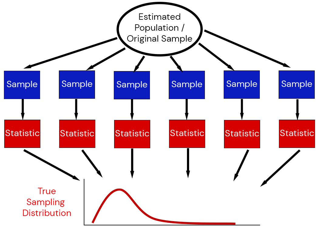
Illustration of the Sampling Distribution
How do we “fit” distributions to a dataset?
Likelihood of data to have come from distribution \(\mathcal{D}\) with pdf \(f(\mathbf{x} | \theta)\):
\[\mathcal{L}(\theta | \mathbf{x}) = \underbrace{f(\mathbf{x} | \theta)}_{\text{PDF}}\]
In other words: likelihood evaluates parameters conditional on data, PDF evaluates data conditional on parameters.
\[f_\mathcal{D}(x) = p(x | \mu, \sigma) = \frac{1}{\sigma\sqrt{2\pi}} \exp\left(-\frac{1}{2}\left(\frac{x - \mu}{\sigma}^2\right)\right)\]
For multiple (independent) samples \(\mathbf{x} = \{x_1, \ldots, x_n\}\):
\[\mathcal{L}(\theta | \mathbf{x}) = \prod_{i=1}^n \mathcal{L}(\theta | x_i).\]
| Distribution | Likelihood |
|---|---|
| \(N(0, 1)\) | 3.7e-11 |
| Distribution | Likelihood |
|---|---|
| \(N(0, 1)\) | 3.7e-11 |
| \(N(-1, 2)\) | 5.9e-10 |
| Distribution | Likelihood |
|---|---|
| \(N(0, 1)\) | 3.7e-11 |
| \(N(-1, 2)\) | 5.9e-10 |
| \(N(-1, 1)\) | 1.2e-13 |
Likelihoods get very small very fast due to multiplying small numbers.
This is a computational problem due to underflow.
We use logarithms to avoid these issues: compute \(\log \mathcal{L}(\theta | x)\).

Next Week: Exploratory Data Analysis
Homework 1 due next Friday (2/6).
Reading: