Code
5×7 DataFrame
| Row | rownames | Ozone | Solar | Wind | Temp | Month | Day |
|---|---|---|---|---|---|---|---|
| Int64 | Int64? | Int64? | Float64 | Int64 | Int64 | Int64 | |
| 1 | 1 | 41 | 190 | 7.4 | 67 | 5 | 1 |
| 2 | 2 | 36 | 118 | 8.0 | 72 | 5 | 2 |
| 3 | 3 | 12 | 149 | 12.6 | 74 | 5 | 3 |
| 4 | 4 | 18 | 313 | 11.5 | 62 | 5 | 4 |
| 5 | 5 | missing | missing | 14.3 | 56 | 5 | 5 |
Lecture 03
January 28, 2026
But not all models are theoretically justifiable.


Source: Richard McElreath
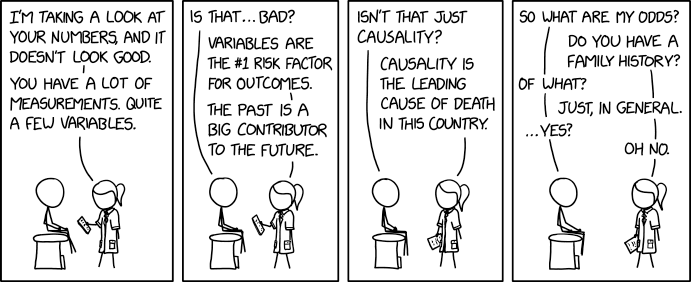
XKCD 2620
Source: XKCD 2620
Four datasets, all with the same means, variances, correlations, and regression lines.
Shows the importance of visualization!

Source: Wikipedia
Boxplots: Show quantiles (usually median + 1.5 \(\times\) IQR)
Histogram: See distribution of data.
# this uses the dataframe plotting syntax from StatsPlots.jl
p1 = @df aq scatter(:Ozone, :Solar, markersize=5, color=:blue, xlabel="Ozone (ppb)", ylabel="Solar Radiation (lang)", leftmargin=10mm)
p2 = @df aq scatter(:Ozone, :Wind, markersize=5, color=:blue, xlabel="Ozone (ppb)", ylabel="Wind Speed (mph)", leftmargin=10mm)
p3 = @df aq scatter(:Ozone, :Temp, markersize=5, color=:blue, xlabel="Ozone (ppb)", ylabel="Max Temperature (°F) ", leftmargin=10mm)

p = plot(p1, p2, p3, layout=(1, 3), size=(1100, 400))
Figure 2: Paired plots of air quality dataset
If we have a candidate distribution, we can try to fit it to the data and visually compare to a histogram.

Here we might try a Log-Normal distribution.

Figure 6: Diagnosing Problems With Q-Q Plots

Figure 7: Diagnosing Problems With Q-Q Plots

Figure 8: Diagnosing Problems With Q-Q Plots

Figure 9: Diagnosing Problems With Q-Q Plots


p1 = qqplot(LogNormal, collect(skipmissing(aq[!, :Ozone])), linewidth=3, markersize=6, title="Log-Normal Q-Q Plot", leftmargin=5mm)
xlabel!(p1, "Theoretical Values")
ylabel!(p1, "Empirical Values")
plot!(pozone, xlims=(0, 300))
p3 = boxplot([ln_samps[1:116] collect(skipmissing(aq[!, :Ozone]))], xlabel="Ozone (ppb)")
xticks!(p3, [1, 2], ["LogNormal", "Ozone Data"])
plot(p1, pozone, p3, layout=(1, 3), size=(1250, 525), rightmargin=5mm, leftmargin=5mm)
Figure 11: QQ Plot comparing ozone data with LogNormal distribution


