AR(1) Inference

Lecture 12

February 20, 2026

Review

Time Series

Dependence: History or sequencing of the data matters

\[p(y_t) = f(y_1, \ldots, y_{t-1})\]

Serial dependence captured by autocorrelation:

\[\varsigma(i) = \rho(y_t, y_{t-i}) = \frac{\text{Cov}[y_t, y_{t+i}]}{\mathbb{V}[y_t]} \]

Figure 1: Autocorrelation for the Lynx data.

AR(1) Models

AR(p): (autoregressive of order \(p\)):

\[ \begin{align*} y_t &= \alpha + \rho y_{t-1} + \varepsilon_t \\ \varepsilon &\sim \mathcal{D}(\theta) \\ y_0 &\sim \mathcal{G}(\psi) \end{align*} \]

\(\mathbb{E}[\varepsilon] = 0\), \(\text{cor}(\varepsilon_i, \varepsilon_j) = 0\), \(\text{cor}(\varepsilon_i, y_0) = 0\)

AR(1) Models

Have memory of autocorrelation even though it’s only explicit for 1 lag.
Weakly stationary if and only if autoregression coefficient \(|\rho| < 1\).
Use partial autocorrelation function to identify lag-1 autocorrelation.

AR(1) Inference

AR(1) Joint Distribution

Assume stationarity and zero-mean process (\(\alpha = 0\)).

Need to know \(\text{Cov}[y_t, y_{t+h}]\) for arbitrary \(h\).

\[ \begin{align*} \text{Cov}[y_t, y_{t-h}] &= \text{Cov}[\rho^h y_{t-h}, y_{t-h}] \\ &= \rho^h \text{Cov}[y_{t-h}, y_{t-h}] \\ &= \rho^h \frac{\sigma^2}{1-\rho^2} \end{align*} \]

AR(1) Joint Distribution

\[ \begin{align*} \mathbf{y} &\sim \mathcal{N}(\mathbf{0}, \Sigma) \\ \Sigma &= \frac{\sigma^2}{1 - \rho^2} \begin{pmatrix}1 & \rho & \ldots & \rho^{T-1} \\ \rho & 1 & \ldots & \rho^{T-2} \\ \vdots & \vdots & \ddots & \vdots \\ \rho^{T-1} & \rho^{T-2} & \ldots & 1\end{pmatrix} \end{align*} \]

Alternatively..

An “easier approach” (often more numerically stable) is to whiten the series sample/compute likelihoods in sequence:

\[ \begin{align*} y_0 & \sim N\left(0, \frac{\sigma^2}{1 - \rho^2}\right) \\ y_t &\sim N(\rho y_{t-1} , \sigma^2) \end{align*} \]

Code for AR(1) model

function ar1_loglik_whitened(θ, dat)
    # might need to include mean or trend parameters as well
    # subtract trend from data to make this mean-zero in this case
    ρ, σ = θ
    T = length(dat)
    ll = 0 # initialize log-likelihood counter
    for i = 1:T
        if i == 1
            ll += logpdf(Normal(0, sqrt(σ^2 / (1 - ρ^2))), dat[i])
        else
            ll += logpdf(Normal(ρ * dat[i-1], σ), dat[i])
        end
    end
    return ll
end

function ar1_loglik_joint(θ, dat)
    # might need to include mean or trend parameters as well
    # subtract trend from data to make this mean-zero in this case
    ρ, σ = θ
    T = length(dat)
    # compute all of the pairwise lags
    # this is an "outer product"; syntax will differ wildly by language
    H = abs.((1:T) .- (1:T)')
    P = ρ.^H # exponentiate ρ by each lag
    Σ = σ^2 / (1 - ρ^2) * P
    ll = logpdf(MvNormal(zeros(T), Σ), dat)
    return ll
end

AR(1) Example

Code

ρ = 0.6
σ = 0.25
T = 25
ts_sim = zeros(T)
# simulate synthetic AR(1) series
for t = 1:T
    if t == 1
        ts_sim[t] = rand(Normal(0, sqrt(σ^2 / (1 - ρ^2))))
    else
        ts_sim[t] = rand(Normal(ρ * ts_sim[t-1], σ))
    end
end

plot(1:T, ts_sim, linewidth=3, xlabel="Time", ylabel="Value", title=L"$ρ = 0.6, σ = 0.25$")
plot!(size=(600, 500))

Code

lb = [-0.99, 0.01]
ub = [0.99, 5]
init = [0.6, 0.3]

optim_whitened = Optim.optimize(θ -> -ar1_loglik_whitened(θ, ts_sim), lb, ub, init)
θ_wn_mle = round.(optim_whitened.minimizer; digits=2)
@show θ_wn_mle;

optim_joint = Optim.optimize(θ -> -ar1_loglik_joint(θ, ts_sim), lb, ub, init)
θ_joint_mle = round.(optim_joint.minimizer; digits=2)
@show θ_joint_mle;

θ_wn_mle = [0.62, 0.23]
θ_joint_mle = [0.62, 0.23]

Dealing with Trends

AR(1) with Trend

\[y_t = \underbrace{x_t}_{\text{fluctuations}} + \underbrace{z_t}_{\text{trend}}\]

Model trend with regression: \[y_t - (a + bt) \sim N(\rho (y_{t-1} - (a + b(t-1))), \sigma^2)\]
Model the spectrum (frequency domain, for periodic trends).
Difference values (integrated time series model): \(\hat{y}_t = y_t - y_{t-1}\)

Be Cautious with Detrending!

Dragons: Extrapolating trends identified using “curve-fitting” is highly fraught, complicating projections.

Better to have an explanatory model and then fit autoregressive models to the residuals…

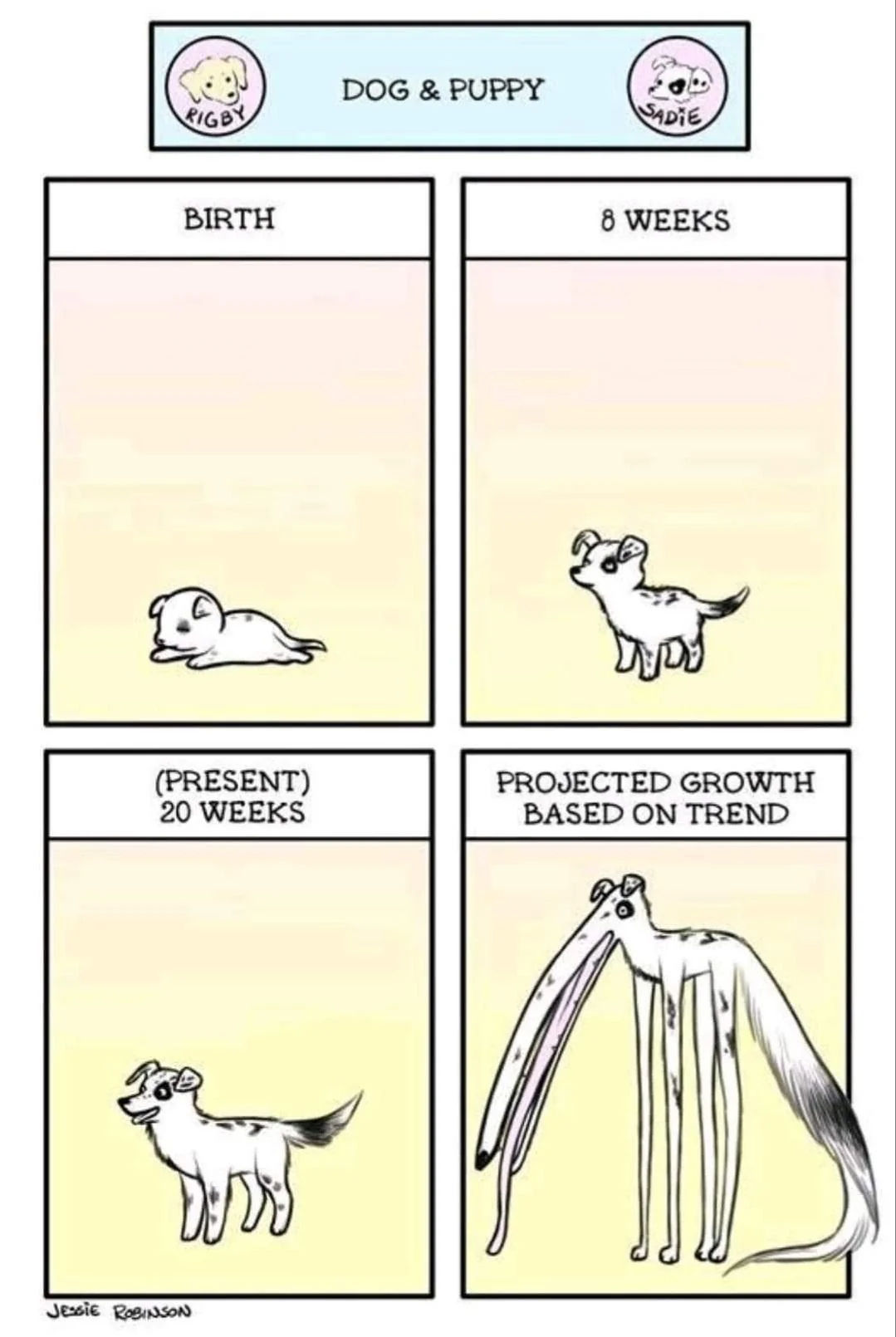
Source: Reddit (original source unclear…)

Sea-Level Rise Example

Figure 3: Global mean sea level and temperature data for Problem 1.

SLR Autocorrelation

Code

pacf_slr = pacf(sl_dat[!, :GMSLR], 0:5)

p1 = plot(0:5, autocor(sl_dat[!, :GMSLR], 0:5), marker=:circle, line=:stem, linewidth=3, markersize=8, legend=false, ylabel="Autocorrelation", xlabel="Time Lag", size=(550, 500))
p2 = plot(0:5, pacf_slr, marker=:circle, line=:stem, markersize=8, linewidth=3, legend=false, ylabel="Partial Autocorrelation", xlabel="Time Lag", size=(550, 500))

display(p1)
display(p2)

SLR Model

Simple model of sea-level rise from Grinsted et al. (2010):

\[\begin{aligned} \frac{dS}{dt} &= \frac{S_\text{eq} - S}{\tau} \\ S_\text{eq} &= aT + b, \end{aligned} \]

Models and Autocorrelation

Note: Hypothetically this type of model can capture all of the autocorrelation (or at least non-stationarity) in the data, since:

the forcings (\(T\)) are autocorrelated;
the differential equation models \(dS/dt\) as a function of \(S\).

So a good strategy is to try to calibrate this model without assuming AR(1) residuals, then see if they’re necessary (HW3).

Model Discretization

Many ways to discretize model, we use the simplest (forward Euler) based on \(\frac{dy}{dx} = \lim_{\Delta x \to 0} \frac{y(x + \Delta x) - y(x)}{\Delta x}\):

Replace \(\frac{dS}{dt}\) with \(\frac{S(t + \Delta t)}{\Delta t}\) for some small time step \(\Delta t > 0\) (here take \(\Delta t = 1\) yr)
Solve for \(S(t + \Delta t)\).

Discrete SLR Model

\[ \begin{aligned} \frac{S(t+1) - S(t)}{\Delta t} &= \frac{S_\text{eq}(t) - S(t)}{\tau} \\[0.5em] S_\text{eq}(t) &= a T(t) + b, \\[1.5em] \Rightarrow S(t+1) &= S(t) + \Delta t \frac{S_\text{eq}(t) - S(t)}{\tau} \\[0.5em] S_\text{eq}(t) &= a T(t) + b, \end{aligned} \]

From Numerical to Probability Model

We can treat this like any other regression, but use model for \(S(t)\) instead of e.g. linear model:

Assuming i.i.d. Gaussian residuals: \[y_t = S(t) + \varepsilon_t, \qquad \varepsilon_t \sim N(0, \sigma^2)\]

If residuals are autocorrelated: \[y_t = S(t) + \omega_t, \quad \omega_t = \rho \omega_{t-1} + \varepsilon_t, \quad \varepsilon_t \sim N(0, \sigma^2)\]

General Idea of Workflow

For a given set of parameters:

Evaluate numerical model to get predictions \(S(t)\);
Calculate residuals \(r(t) = y(t) - S(t)\);
Maximize likelihood of residuals according to probability model.

Model Discrepancy

Can go further and separate out observation errors (typically white noise) from model-data discrepancies (systematic differences in state prediction, often autocorrelated):

Computer Model: \[\eta(\underbrace{\theta}_{\substack{\text{calibration}\\\text{variables}}}; \underbrace{x}_{\substack{\text{control}\\\text{variables}}})\]

Observations: \[\mathbf{y} \sim p(\underbrace{\zeta(\mathbf{x})}_{\substack{\text{expected}\\\text{state}}})\]

Model-Data Discpreancy

Write \[\zeta(\mathbf{x}) = \delta(\eta(\theta; x))\] where \(\delta\) represents the discrepancy between the model output and the expected state.

Then the probability model is: \[\mathbf{y} \sim p(\delta(\eta(\theta; x))).\]

Most common setting (e.g. Brynjarsdóttir & O’Hagan (2014)):

\[\mathbf{y} = \underbrace{\eta(\mathbf{x}; \theta)}_{\text{model}} + \underbrace{\delta(x)}_{\text{discrepancy}} + \underbrace{\varepsilon}_{\text{error}}\]

Higher Order Autoregressions

AR(p)

\[y_t = a + \rho_1 y_{t-1} + \rho_2 y_{t-2} + \ldots + \rho_p y_{t-p} + \varepsilon_t\]

Same basic ideas, but more difficult to estimate and easy to overfit.
Simulate/predict by sampling first \(p\) values and innovations, then plug into equation.
Can have much more interesting dynamics, including oscillations.

Key Points

Can do inference for AR(1) either by whitening residuals or fitting joint distribution.
Often numerical models have autocorrelated residuals: this can produce very different estimates than assuming independent Gaussian residuals.
Common problem when fitting models by minimizing (R)MSE!

For More On Time Series

Courses

STSCI 4550/5550 (Applied Time Series Analysis),
CEE 6790 (heavy focus on spectral analysis and signal processing)

Books

Shumway & Stoffer (2025)
Hyndman & Athanasopoulos (2021)
Durbin & Koopman (2012)
Banerjee et al. (2011)
Cressie & Wikle (2011)

Upcoming Schedule

Next Classes

Next Week: Extreme Values (Theory and Models)

Next Unit: Hypothesis Testing, Model Evaluation, and Comparison

Assessments

HW2: Due Friday at 9pm.

Exercises: Available after class (will include GLMs + time series).

HW3: Assigned on 3/2, due 3/13.

References

References (Scroll For Full List)

Banerjee, S., Carlin, B. P., & Gelfand, A. E. (2011). Hierarchical modeling and analysis for spatial data, second edition (2nd ed.). Philadelphia, PA: Chapman & Hall/CRC. https://doi.org/10.1201/b17115

Brynjarsdóttir, J., & O’Hagan, A. (2014). Learning about physical parameters: the importance of model discrepancy. Inverse Problems, 30, 114007. https://doi.org/10.1088/0266-5611/30/11/114007

Cressie, N., & Wikle, C. K. (2011). Statistics for Spatio-Temporal Data. Hoboken, NJ: Wiley.

Durbin, J., & Koopman, S. J. (2012). Time series analysis by state space methods (2nd ed.). London, England: Oxford University Press. https://doi.org/10.1093/acprof:oso/9780199641178.001.0001

Grinsted, A., Moore, J. C., & Jevrejeva, S. (2010). Reconstructing sea level from paleo and projected temperatures 200 to 2100 ad. Clim. Dyn., 34, 461–472. https://doi.org/10.1007/s00382-008-0507-2

Hyndman, R. J., & Athanasopoulos, G. (2021). Forecasting: Principles and Practice (3rd ed). Melbourne, Australia: OTexts. Retrieved from https://otexts.com/fpp3/

Shumway, R. H., & Stoffer, D. S. (2025). Time series analysis and its applications. Springer.