(Null) Hypothesis Testing

---

Lecture 22

March 16, 2026

Overview

• Review
• Statistical Significance
• Problems with Null Hypothesis Testing
• Key Points
• Upcoming Schedule
• References

Review

Questions We Might Like To Answer

• Are high water levels influenced by environmental change?
• Does some environmental condition have an effect on water quality/etc?
• Does a drug or treatment have some effect?

Each of these is a hypothesis about causation or influence.

Null Hypothesis Significance Testing

• Check if the data is consistent with a “null” model;
• If the data is unlikely from the null model (to some level of significance), this is evidence for the alternative.
• If the data is consistent with the null, there is no need for an alternative hypothesis.

Alternative Hypothesis Meme

For scientific hypotheses, this has been encoded in the NHST paradigm:

• Think of a “null” hypothesis and look for evidence that it is reasonably consistent with the data.
• If the data can be explained by the null, then we have no clear evidence for the alternative hypothesis.
• If the data is highly unlikely under the null hypothesis, then that gives us reason to reject the null and favor the alternative.

p-Values: Quantification of “Surprise”

One-Tailed Test:

Figure 1: Illustration of a p-value

Two-Tailed Test:

Figure 2: Illustration of a two-tailed p-value

Statistical Significance

Error Types

		Null Hypothesis Is
		True	False
Decision About Null Hypothesis	Don’t reject	True negative (probability \(1-\alpha\))	Type II error (probability \(\beta\))
	Reject	Type I Error (probability \(\alpha\))	True positive (probability \(1-\beta\))

The general testing framework is built around Type I (false positive) and Type II (false negative) errors.

Navigating Type I and II Errors

The standard null hypothesis significance framework is based on balancing the chance of making Type I (false positive) and Type II (false negative) errors.

Idea: Set a significance level \(\alpha\) which is an “acceptable” probability of making a Type I error.

Aside: The probability \(1-\beta\) of correctly rejecting \(H_0\) is the power.

Note that these are frequentist concepts, not applicable to a single dataset (which give rise to p-values, which are random values).

If we only run a single experiment all we can claim is that if we had run a long series of experiments we would have had 100α% false positives had H0 been true and 100β% false negatives had H1 been true provided we got the power calculations right. Note the conditionals.

p-Value and Significance

Common practice: If the p-value is sufficiently small (below \(\alpha\)), reject the null hypothesis with \(1-\alpha\) confidence, or declare that the alternative hypothesis is statistically significant at the \(1-\alpha\) level.

This can mean:

1. The null hypothesis is not true for that data-generating process;
2. The null hypothesis is true but the data is an outlying sample.

This is a strange hybrid of two schools of frequentist statistics, that of Fisher and of Neyman-Pearson. Fisher viewed p-values as weak evidence which was part of an inductive process (even when assuming unbiased sampling and accurate measurement), while the Neyman-Pearson significance framework was based on quantitative specifications of alternative hypotheses with explicitly calculated power.

What p-Values Are Not

1. Probability that the null hypothesis is true (this is never computed);
2. An indication of the effect size (or the stakes of that effect).

\[ \underbrace{p(S \geq \hat{S}) | \mathcal{H}_0)}_{\text{p-value}} \neq \underbrace{p(\mathcal{H}_0 | S \geq \hat{S})}_{\substack{\text{probability of} \\ \text{null}}}!\]

A p-value is a random variable which depends on the data. It’s evidence which can be collected from a single experiment but can not establish truth.

Over repeated experiments, reasoning about validity of the null should have the right properties assuming the experiments are conducted faithfully.

Problems with Null Hypothesis Testing

What Is Included In Statistical Significance?

1. Is the model right?
2. Did I estimate the parameter correctly?
3. Conditional on the model being right and my estimation being right, could the data have come from

Statistical Significance ≠ Scientific Significance

After a test like whether \(\beta = 0\) or not, it is common to hear people say something like “\(\beta\) is [statistically] significant.”

This is true in a technical sense, but e.g. non-rejection of the null hypothesis does not mean that \(\beta\) is trivial or can be ignored.

Why?

Why Might A Null Be Retained?

1. \(\beta = 0\) in reality;
2. \(\beta \neq 0\) but the standard errors are large and zero is within them.

For example: \(\beta\) can be quite large, but with large standard errors, and the null hypothesis would be retained.

You actually need to look at the sampling distribution/confidence intervals to know this!

Statistical Significance ≠ Scientific Significance

Statistical significance mixes together a number of different concepts:

1. How big is the coefficient?
2. How big is the sample?
3. How much noise is there around the regression line;
4. How spread out is the data along the \(x\)-axis?

Statistical Significance ≠ Scientific Significance

Statistical significance also does not mean anything about whether the alternative hypothesis is:

1. “true”;
2. an accurate reflection of the data-generating process.

Hypothesis vs. Causal Meme

What is Any Statistical Test Doing?

1. Assume the null hypothesis \(\mathcal{H}_0\).
2. Compute the test statistic \(\hat{S}\) for the sample.
3. Obtain the sampling distribution of the test statistic \(S\) under \(H_0\).
4. Calculate \(\mathbb{P}(S > \hat{S})\) (the p-value).

A Parametric Test Statistic for Non-Stationarity

Fit a regression

\[ \begin{gather*} y_i = \beta_0 + \beta_1 t + \varepsilon_i, \\ \varepsilon_i \sim \mathcal{N}(0, \sigma^2\mathbb{I}). \end{gather*} \]

SF Tide Gauge Data: \((\hat{\beta}_0, \hat{\beta}_1) \approx (1.26, 4 \times 10^{-4})\)

Parametric Null Hypothesis

\(\mathcal{H}_0: \beta_1 = 0\)

Use the \(t\)-statistic:

\[\hat{t} = \frac{\hat{\beta_1}}{se(\hat{\beta_1)}}, \quad \hat{t} \sim t_{n-2}.\]

SF Data: \(\hat{t} = 2.31\), \(p\text{-value} \approx 0.01\).

(a) Test statistic and null distribution for surge stationary detection with a linear regression.

(b)

Figure 3

Non-Parametric Test for Non-Stationary

A non-parametric alternative is the Mann-Kendall Test:

Assume data is independent and no periodic signals, but no specific distributional assumption. Test statistic \(S\):

\[S = \sum_{i=1}^{n-1} \sum_{j={1+1}}^n \text{sgn}\left(y_j - y_i\right).\]

SF Tide Gauge Data: \(S=921\).

Non-Parametric Null Hypothesis

\(\mathcal{H}_0: S = 0\) (no average trend).

The null sampling distribution of \(S\) is \(N(0, \sqrt{\text{Var}(S)})\), where \[\text{Var}(S) = \frac{n(n-1)(2n+5)}{18} - \sum_{i=1}^g t_i(t_i - 1)(2t_i + 5),\]

\(g\) are the number of equal values and \(t_i\) is the size of tie group \(i\)

SF Tide Gauge Data: \(Var(S) = 224875\)

Difference in \(p\)-Values

Is there a trend in the SF tide gauge trend data?

• Trend as regression (\(p\text{-value} \approx 0.01\))
• Mann-Kendall test for monotonic trend (\(p\text{-value} \approx 0.03\))

Non-Uniqueness of Null Models

Source: McElreath (2020, fig. 1.2)

Multiple Comparisons

If you conduct multiple statistical tests, you must account for all of these in the p-value computation and assessment of significance.

Multiple Comparisons Meme

Multiple Comparisons

For example: an appropriate applied test at a 5% significance level will result in a 5% Type I error rate. But if you do 100 independent tests, the Type I rate is 99.4%!

Multiple Comparisons Meme

The core issue is the standard test statistics have the right Type I/Type II properties for each individual test, but multiple tests distort these frequencies, sometimes quite dramatically.

For example, suppose each individual test has a 5% Type I error rate. If you test 100 different models, and the errors are independent, you would expect 5 false positives, one of which would be selected by minimizing the p-value. The probability of at least one type I error is >99%.

There are a number of corrections (Bonferroni being the most common), but sometimes stepwise tests are subtle, including cases of model selection followed by model fitting. You can also use simulation to estimate the false-positive rate for the procedure under a null data-generating process, which ties into the broader methods we’ll discuss.

Results Are Flashy, But Meaningless Without Methods

Elton John Results Section Meme

Source: Richard McElreath

Note: This Does Not Mean Null Hypothesis Testing Is Useless!

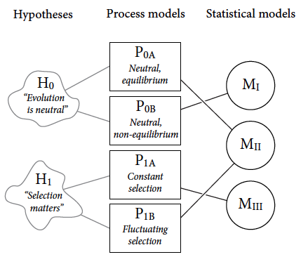
Examining and testing the implications of competing models is important, including “null” models!

Null Hypothesis Selection Good Vs. Bad

Deborah Mayo discusses this interpretation as “severe testing”: apply different levels of scrutiny to a scientific model to see what level of severity breaks the model.

The idea of a p-value (not necessarily “significance”) being a piece of inductive evidence rather than a threshold for validity (especially for an individual experiment) reflects the original views of Fisher.

What Can We Do Instead?

Use computing for simulation:

1. Develop sampling distributions and confidence intervals for more arbitrary models which reflect meaningful hypotheses about data-generating processes;
2. Compare model predictive performance involving models chosen based on scientific hypotheses.
3. When desired, compute \(p\)-values (including for multiple comparisons) by simulating Type I error rates.

Key Points

Hypothesis Testing

• Classical framework: Compare a null hypothesis (no effect) to an alternative (some effect)
• \(p\)-value: probability (under \(H_0\)) of more extreme test statistic than observed.
• “Significant” if \(p\)-value is below a significance level reflecting acceptable Type I error rate.

Problems with NHST framework

• Real “null” hypotheses are often more nuanced than in typical tests (which were often developed for controlled experiments or for computational convenience).
• Decisions are often not binary (“significant/not significant”).
• \(p\)-values are often over-interpreted and are often be incorrectly calculated, with negative outcomes!
• Important: “Big” data can make things worse, as NHST is highly sensitive to small but evidence effects.

Upcoming Schedule

Next Classes

Wednesday: Introduction to Simulation and Random Sampling

Friday: Sampling and Monte Carlo

Next Week The Bootstrap

Assessments

HW4 assigned, due 3/27.

References

References (Scroll for Full List)

McElreath, R. (2020). Statistical rethinking : A bayesian course with examples in R and Stan (Second). Boca Raton, Florida: CRC. Retrieved from https://www.routledge.com/Statistical-Rethinking-A-Bayesian-Course-with-Examples-in-R-and-STAN/McElreath/p/book/9780367139919