
Simulating Random Variables
Lecture 23
March 20, 2026
Using the PDF
Suppose the PDF \(f\) has support on \([a, b]\) and \(f(x) \leq M\).
What could we do to sample \(X \sim f(\cdot)\)?
Rejection Sampling Visualization

Figure 2: Example of rejection sampling for a Beta distribution
Rejection Sampling Efficiency
Important: Only kept 28% of proposals.


More General Rejection Sampling
Use a proposal density \(g(\cdot)\) which “covers” target \(f(\cdot)\) and is easy to sample from.
Sample from \(g\), reject based on \(f\).

Rejection Sampling Example

This time we kept 34% of the proposals.
Bimodal Rejection Sampling Example
Code
# specify target distribution
mixmod = MixtureModel(Normal, [(-1, 0.75), (1, 0.4)], [0.5, 0.5])
x = -5:0.01:5
p1 = plot(x, pdf.(mixmod, x), lw=3, color=:red, xlabel=L"$x$", ylabel="Density", label="Target")
plot!(p1, x, 2.5 * pdf.(Normal(0, 1.5), x), lw=3, color=:blue, label="Proposal (M=2.5)")
plot!(p1, size=(550, 500))

nsamp = 10_000
M = 2.5
u = rand(Uniform(0, 1), nsamp)
y = rand(Normal(0, 1.5), nsamp)
g = pdf.(Normal(0, 1.5), y)
f = pdf.(mixmod, y)
keep_samp = u .< f ./ (M * g)
p2 = histogram(y[keep_samp], normalize=:pdf, xlabel=L"$x$", ylabel="Density", label="Kept Samples", legend=:topleft)
plot!(p2, x, pdf.(mixmod, x), linewidth=3, color=:black, label="True Target")
density!(y[keep_samp], label="Sampled Density", color=:red)
plot!(p2, size=(550, 500))

display(p1)
display(p2)

Where Do “Random” Samples Come From?
There’s no such thing as a truly random number generator!
Need to generate samples in a deterministic way that have random-like properties.
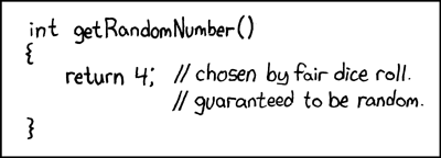
Source: XKCD 221
Example: Arnold Cat Map
\[ \begin{align*} \phi_{t+1} &= 2U_t + \phi_t \mod 1 \\ U_{t+1} &= \phi_t + U_t \mod 1 \end{align*} \]
Report only \((U_t)\): get hard to predict uniformly distributed data.

Source: Wikipedia
Cat Map vs Mersenne Twister
Code
function cat_map(N)
    U = zeros(N)
    ϕ = zeros(N)
    U[1], ϕ[1] = rand(Uniform(0, 1), 2)
    for i = 2:N
        ϕ[i] = rem(U[i-1] + 2 * ϕ[i-1], 1.0)
        U[i] = rem(U[i-1] + ϕ[i-1], 1.0)
    end
    return U
end

N = 1_000
Z = cat_map(N)
U = rand(MersenneTwister(1), N) # Mersenne Twister is not the default in Julia, but is in other languages, so using it here by explicitly setting it as the generator

p1 = scatter(Z[1:end-1], Z[2:end], xlabel=L"$U_t$", ylabel=L"$U_{t+1}$", title="Cat Map", label=false, size=(500, 500))
p2 = scatter(U[1:end-1], U[2:end], xlabel=L"$U_t$", ylabel=L"$U_{t+1}$", title="Mersenne Twister", label=false, size=(500, 500))

display(p1)
display(p2)
