So Far…
We’re 12 weeks in and haven’t said anything about how to quantify uncertainties in model estimation.
Let’s talk about that.
Implications of Sampling Variability
- The data is one realization of a stochastic process.
- Estimates of statistical quantities (parameters, test statistics, etc) depend on the data.
- If we were to “re-run the tape”, we would get different data, and therefore different estimates.
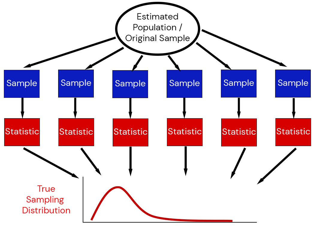
How To Quantify Sampling Variability
- Standard errors: how much would we expect this quantity to vary from one data replication to another?
- Confidence intervals: what are the parameters that might have been expected to produce this data with some pre-assigned probability?
But for both of these, we need to know the sampling distribution: the underlying distribution of estimates across different data replications.
Sampling Distributions
The sampling distribution of a statistic captures the uncertainty associated with random samples.
Estimating Sampling Distributions
- Special Cases: can derive closed-form representations of sampling distributions (think statistical tests)
- Asymptotics: Central Limit Theorem or Fisher Information
Special Case: Linear Regression
Theory around linear regression: if data is truly generated by some linear model (or something reasonable close), then
\[\frac{\hat{\beta} - \beta}{\hat{\text{se}}\left[\hat{\beta}\right]} \sim t_{n-2}\]
This means that even if the model is correctly specified, the standardized estimates of a coefficient \(\beta\) can be expected to follow a \(t\) distribution based on sampling variability.
Next Classes
Wednesday: The Nonparametric Bootstrap
Friday: The Parametric Bootstrap
Assessments
Homework 5: Due next Friday (4/17)
Project Updates: Due Friday (4/10)
Quiz 3: Friday (4/10) through pre-break material on Monte Carlo.