Code
1×20 adjoint(::Vector{Bool}) with eltype Bool:
1 1 0 0 0 1 0 0 0 1 1 1 1 1 1 0 1 1 1 1
Lecture 28
April 8, 2026
But for both of these, we need to know the sampling distribution: the underlying distribution of estimates across different data replications.
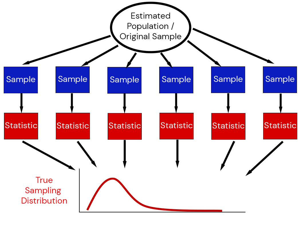
The sampling distribution of a statistic captures the uncertainty associated with random samples.

This means we need:
Efron (1979) suggested combining estimation with simulation: the bootstrap.
Key idea: use the data to simulate a data-generating mechanism.


Efron’s key insight: due to the Central Limit Theorem, the bootstrap distribution \(\mathcal{D}(\tilde{t}_i)\) has the same relationship to the observed estimate \(\hat{t}\) as the sampling distribution \(\mathcal{D}(\hat{t})\) has to the “true” value \(t_0\):
\[\mathcal{D}(\tilde{t} - \hat{t}) \approx \mathcal{D}(\hat{t} - t_0)\]
where \(t_0\) the “true” value of a statistic, \(\hat{t}\) the sample estimate, and \((\tilde{t}_i)\) the bootstrap estimates.
In other words:
The population is to the sample what the sample is to the bootstrap samples.
Let \(t_0\) the “true” value of a statistic, \(\hat{t}\) the estimate of the statistic from the sample, and \((\tilde{t}_i)\) the bootstrap estimates.
Notice that bias correction “shifts” away from the bootstrapped samples.
Suppose we want to construct a \(1-\alpha\)% CI for \(t_0\). The most naive application of the bootstrap principle suggests that with \(1-\alpha\)% probability, then \(t_0\) falls inbetween \(Q_{\tilde{t}}(\alpha/2)\) and \(Q_{\tilde{t}}(1-\alpha/2))\).
Therefore, if the distribution for \(\tilde{t}\) approximates the sampling distribution of \(\hat{t}\), we get the:
Percentile Bootstrap CI: \[(Q_{\tilde{t}}(\alpha/2), Q_{\tilde{t}}(1-\alpha/2))\]
The assumption that \(\mathcal{D}(\tilde{t}) \approx \mathcal{D}(\hat{t})\) is pretty strong and generally not satisfied! Instead, suppose it’s only the variability in the samples that we assume is similar, e.g. \[\mathcal{D}(\tilde{t} - \hat{t}) \approx \mathcal{D}(\hat{t} - t_0)\].
Then:
\[\begin{aligned} 1 - \alpha &= \mathbb{P}\left[Q_{\tilde{t}}(\alpha/2) \leq \tilde{t} \leq Q_{\tilde{t}}(1 - \alpha/2) \right] \\ &= \mathbb{P}\left[Q_{\tilde{t}}(\alpha/2) - \hat{t} \leq \tilde{t} - \hat{t} \leq Q_{\tilde{t}}(1 - \alpha/2) - \hat{t} \right] \\ &= \mathbb{P}\left[\hat{t} - Q_{\tilde{t}}(\alpha/2) \geq \color{red}{\hat{t} - \tilde{t}} \geq \hat{t} - Q_{\tilde{t}}(1 - \alpha/2) \right] \\ &\approx \mathbb{P}\left[\hat{t} - Q_{\tilde{t}}(\alpha/2) \geq \color{red}{t_0 - \hat{t}} \geq \hat{t} - Q_{\tilde{t}}(1 - \alpha/2) \right] \\ &= \mathbb{P}\left[2\hat{t} - Q_{\tilde{t}}(\alpha/2) \geq t_0 \geq 2\hat{t} - Q_{\tilde{t}}(1 - \alpha/2) \right] \end{aligned}\]
This gives us the:
Basic Bootstrap CI: \(\left(2\hat{t} - Q_{\tilde{t}}(1-\alpha/2), 2\hat{t} - Q_{\tilde{t}}(\alpha/2)\right)\)
Suppose there is a bias \(\mathbb{E}\left[\tilde{t}\right] = \bar{t}^* = \hat{t} + B\) and let \[Q_{\tilde{t}}(0.05) = \bar{t}^* - \sigma_1\] and \[Q_{\tilde{t}}(0.95) = \bar{t}^* + \sigma_2.\]
Then the 90% percentile CI is \[\left(\hat{t} + B - \sigma_1, \hat{t} + B + \sigma_2\right)\] while the 90% basic bootstrap CI is
\[\begin{aligned} &\left(2\hat{t} - \left(\bar{t}^* + \sigma_2\right), 2 \hat{t} - \left(\bar{t}^* - \sigma_1\right)\right) \\ &=\left(\hat{t} - B - \sigma_2, \hat{t} - B + \sigma_1\right). \end{aligned}\]
In other words, the percentile CI will get the bias wrong and flip potential assymetries due to skew.
It can be reasonable if you know there is not much bias or skew, but this is hard to guarantee in practice: better to use the basic CI or more advanced CIs (next week).
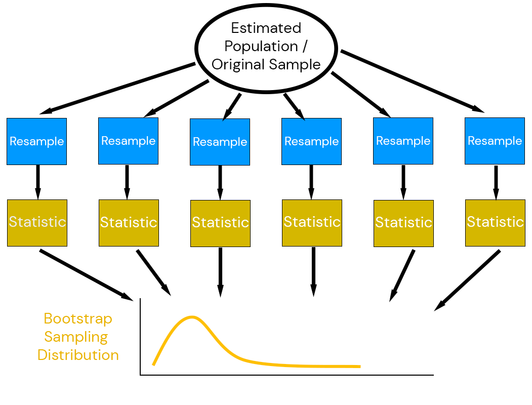
The non-parametric bootstrap is the most “naive” approach to the bootstrap: resample-then-estimate.

Suppose we have observed twenty flips with a coin, and want to know if it is weighted.
1×20 adjoint(::Vector{Bool}) with eltype Bool:
1 1 0 0 0 1 0 0 0 1 1 1 1 1 1 0 1 1 1 1
The frequency of heads is 0.65.
# bootstrap: draw new samples
function coin_boot_sample(dat)
boot_sample = sample(dat, length(dat); replace=true)
return boot_sample
end
function coin_boot_freq(dat, nsamp)
boot_freq = [sum(coin_boot_sample(dat)) for _ in 1:nsamp]
return boot_freq / length(dat)
end
boot_out = coin_boot_freq(dat, 1000)
q_boot = 2 * freq_dat .- quantile(boot_out, [0.975, 0.025])
p = histogram(boot_out, xlabel="Heads Frequency", ylabel="Count", title="1000 Bootstrap Samples", label=false, right_margin=5mm)
vline!(p, [p_true], linewidth=3, color=:orange, linestyle=:dash, label="True Probability")
vline!(p, [mean(boot_out) ], linewidth=3, color=:red, linestyle=:dash, label="Bootstrap Mean")
vline!(p, [freq_dat], linewidth=3, color=:purple, linestyle=:dot, label="Observed Frequency")
vspan!(p, q_boot, linecolor=:grey, fillcolor=:grey, alpha=0.3, fillalpha=0.3, label="95% CI")
plot!(p, size=(1000, 450))Figure 1: Bootstrap heads frequencies for 20 resamples.
n_flips = 50
dat = rand(coin_dist, n_flips)
freq_dat = sum(dat) / length(dat)
boot_out = coin_boot_freq(dat, 1000)
q_boot = 2 * freq_dat .- quantile(boot_out, [0.975, 0.025])
p = histogram(boot_out, xlabel="Heads Frequency", ylabel="Count", title="1000 Bootstrap Samples", titlefontsize=20, guidefontsize=18, tickfontsize=16, legendfontsize=16, label=false, bottom_margin=7mm, left_margin=5mm, right_margin=5mm)
vline!(p, [p_true], linewidth=3, color=:orange, linestyle=:dash, label="True Probability")
vline!(p, [mean(boot_out) ], linewidth=3, color=:red, linestyle=:dash, label="Bootstrap Mean")
vline!(p, [freq_dat], linewidth=3, color=:purple, linestyle=:dot, label="Observed Frequency")
vspan!(p, q_boot, linecolor=:grey, fillcolor=:grey, alpha=0.3, fillalpha=0.3, label="95% CI")
plot!(p, size=(1000, 450))Figure 2: Bootstrap heads frequencies for 1000 resamples.
Generally, anything very sensitive to outliers which might not be re-sampled.
Friday: The Non-Parametric Bootstrap
Next Week: Parametric Bootstrap and Other Nuances
Homework 5: Due next Friday (4/17)
Project Updates: Due Friday (4/10)
Quiz 3: Friday (4/10) through pre-break material on Monte Carlo.