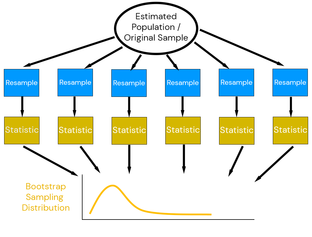
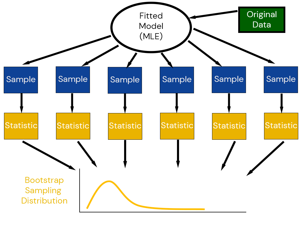
## re-do bootstrap with lognormal distribution
# function to fit GEV model for each data set
init_θ = [1.0, 1.0]
lb = [0.0, 0.0]
ub = [5.0, 10.0]
loglik_ln(θ) = -sum(logpdf(LogNormal(θ[1], θ[2]), dat_annmax.residual))
θ_ln = Optim.optimize(loglik_ln, lb, ub, init_θ).minimizer

boot_samp_ln = rand(LogNormal(θ_ln[1], θ_ln[2]), (nrow(dat_annmax), n_boot))
rp_boot_ln = mapslices(col -> quantile(col, 0.99), boot_samp_ln, dims=1)'
q_boot_ln = 2 * rp_emp .- quantile(rp_boot_ln, [0.975, 0.025])

## plot confidence intervals and estimates
## GEV fit
pfit = plot(GeneralizedExtremeValue(θ_gev[1], θ_gev[2], θ_gev[3]), color=:darkorange, linewidth=3, label="GEV Model", xlabel="Annual Maximum Storm Tide (m)", ylabel="Probability Density", right_margin=5mm)
vline!(pfit, [rp_emp], color=:black, linewidth=3, linestyle=:dash, label="Empirical Return Level")
xlims!(pfit, 1, 1.75)
vline!(pfit, [mean(rp_boot)], color=:orange, linewidth=3, label=false)
vline!(pfit, [2 * rp_emp - mean(rp_boot)], color=:orange, linewidth=3, linestyle=:dot, label=false)
## lognormal fit
plot!(pfit, LogNormal(θ_ln[1], θ_ln[2]), color=:darkgreen, lw=3, label="LogNormal Model")
vline!(pfit, [mean(rp_boot_ln)], color=:green, linewidth=3, label=false)
vline!(pfit, [2 * rp_emp - mean(rp_boot_ln)], color=:green, linewidth=3, linestyle=:dot, label=false)
plot!(pfit, size=(550, 550))

## GEV histogram
phist = histogram(rp_boot, xlabel="100-Year Return Period Estimate (m)", ylabel="Count", right_margin=5mm, legend=false, color=:darkorange, alpha=0.4)
vline!(phist, [2 * rp_emp - mean(rp_boot)], color=:red, linestyle=:dot, linewidth=3)
vspan!(phist, q_boot, linecolor=:orange, fillcolor=:orange, lw=3, alpha=0.3, fillalpha=0.3)
histogram!(phist, rp_boot_ln, fillcolor=:green, alpha=0.3, label="LN Bootstrap Samples")
vline!(phist, [2 * rp_emp - mean(rp_boot_ln)], color=:purple, linestyle=:dot, linewidth=3)
vspan!(phist, q_boot_ln, linecolor=:darkgreen, fillcolor=:darkgreen, lw=3, alpha=0.3, fillalpha=0.3)
plot!(phist, size=(550, 550))

display(pfit)
display(phist)