Hidden Markov Models


Lecture 37

April 29, 2026

Review

Mixture Models

Mixture of Distributions

Mixture model: several different distributions mixed with different weights.

\[\begin{aligned} Z &\sim \text{Mult}(\pi_1, \ldots, \pi_K) \\ Y | Z &\sim \mathcal{D}_Z = f_Z \end{aligned}\]

Very common to use Gaussians for \(\mathcal{D}_k\) but this isn’t necessary.

Mixture Models and Clustering

Mixture models are common for model-based clustering (a parametric alternative to e.g. \(k\)-means).

This is:

  • Good! A mixture model is predictive, might explain the data, and can be checked with e.g. cross-validation.
  • Bad! Highly sensitive to specification of distributions.

E-M Algorithm

Iterative optimization algorithm which alternates between computing the expected log-likelihood given parameter guesses (E-Step) and maximizing that expected log-likelihood to update parameter values (M-Step).

Can directly compute E-Step and M-Step outcomes with Gaussian mixtures.

Otherwise, can use numerical optimization for M-Step and Monte Carlo/other methods for E-Step.

What Don’t Mixture Models Tell Us

Mixture models are useful for clustering or generating bimodel distributions. But they are limited for understanding intertemporal dynamics.

For example: we don’t see the persistence of wet/dry states, with frequent switches between them. Is this reasonable?

To address this, we’ll need a generative model for state switching: a Hidden Markov Model.

Markov Chains

Hidden Markov Models

Instead, we might want to model the process that gives rise to a mixture distribution.

One way to do this for time series is with a Hidden Markov Model where the generative model at time \(t\) probability model “switches” probabilistically based on a Markov chain.

What Is A Markov Chain?

Consider a stochastic process \(\{X_t\}_{t \in \mathcal{T}}\), where

  • \(X_t \in \mathcal{S}\) is the state at time \(t\), and
  • \(\mathcal{T}\) is a time-index set (can be discrete or continuous)
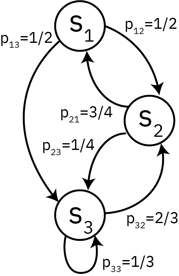
  • \(\mathbb{P}(s_i \to s_j) = p_{ij}\).

Markov State Space

Markovian Property

This stochastic process is a Markov chain if it satisfies the Markovian (or memoryless) property: \[\begin{align*} \mathbb{P}(X_{T+1} = s_i &| X_1=x_1, \ldots, X_T=x_T) = \\ &\qquad\mathbb{P}(X_{T+1} = s_i| X_T=x_T) \end{align*} \]

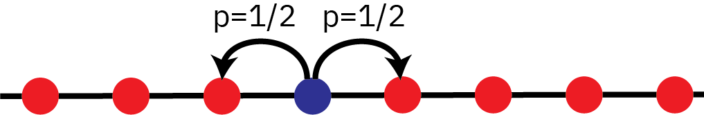
Example: “Drunkard’s Walk”

:img Random Walk, 80%
  • How can we model the unconditional probability \(\mathbb{P}(X_T = s_i)\)?
  • How about the conditional probability \(\mathbb{P}(X_T = s_i | X_{T-1} = x_{T-1})\)?

Example: Weather

Suppose the weather can be foggy, sunny, or rainy.

Based on past experience, we know that:

  1. There are never two sunny days in a row;
  2. Even chance of two foggy or two rainy days in a row;
  3. A sunny day occurs 1/4 of the time after a foggy or rainy day.

Aside: Higher Order Markov Chains

Suppose that today’s weather depends on the prior two days.

  1. Can we write this as a Markov chain?
  2. What are the states?

Weather Transition Matrix

We can summarize these probabilities in a transition matrix \(P\): \[ P = \begin{array}{cc} \begin{array}{ccc} \phantom{i}\color{red}{F}\phantom{i} & \phantom{i}\color{red}{S}\phantom{i} & \phantom{i}\color{red}{R}\phantom{i} \end{array} \\ \begin{pmatrix} 1/2 & 1/4 & 1/4 \\ 1/2 & 0 & 1/2 \\ 1/4 & 1/4 & 1/2 \end{pmatrix} & \begin{array}{ccc} \color{red}F \\ \color{red}S \\ \color{red}R \end{array} \end{array} \]

Rows are the current state, columns are the next step, so \(\sum_i p_{ij} = 1\).

Weather Example: State Probabilities

Denote by \(\lambda^t\) a probability distribution over the states at time \(t\).

Then \(\lambda^t = \lambda^{t-1}P\):

\[\begin{pmatrix}\lambda^t_F & \lambda^t_S & \lambda^t_R \end{pmatrix} = \begin{pmatrix}\lambda^{t-1}_F & \lambda^{t-1}_S & \lambda^{t-1}_R \end{pmatrix} \begin{pmatrix} 1/2 & 1/4 & 1/4 \\ 1/2 & 0 & 1/2 \\ 1/4 & 1/4 & 1/2 \end{pmatrix} \]

Multi-Transition Probabilities

Notice that \[\lambda^{t+i} = \lambda^t P^i,\] so multiple transition probabilities are \(P\)-exponentials.

\[P^3 = \begin{array}{cc} \begin{array}{ccc} \phantom{iii}\color{red}{F}\phantom{ii} & \phantom{iii}\color{red}{S}\phantom{iii} & \phantom{ii}\color{red}{R}\phantom{iii} \end{array} \\ \begin{pmatrix} 26/64 & 13/64 & 25/64 \\ 26/64 & 12/64 & 26/64 \\ 26/64 & 13/64 & 26/64 \end{pmatrix} & \begin{array}{ccc} \color{red}F \\ \color{red}S \\ \color{red}R \end{array} \end{array} \]

Long Run Probabilities

What happens if we let the system run for a while starting from an initial sunny day?

Code
current = [1.0, 0.0, 0.0]
P = [1/2 1/4 1/4
    1/2 0 1/2
    1/4 1/4 1/2]   

T = 21

state_probs = zeros(T, 3)
state_probs[1,:] = current
for t=1:T-1
    state_probs[t+1, :] = state_probs[t:t, :] * P
end


p = plot(0:T-1, state_probs, label=["Foggy" "Sunny" "Rainy"], palette=:mk_8, linewidth=3)
xlabel!("Time")
ylabel!("State Probability")
plot!(p, size=(1000, 350))

Figure 1: State probabilities for the weather examples.

Hidden Markov Models

Hidden Markov Models

A Hidden Markov Model is a model in which a Markov chain gives the latent states \(Z_t\) and \[Y | (Z_t = k) \sim \mathcal{D}_k.\]

Now we need to estimate the:

  • parameters of each emissions distribution \(\mathcal{D}_k\);
  • transition probability matrix \(P\);
  • most probable latent states for each observation (the Viterbi sequence).

Baum-Welch Algorithm

We do this using the Baum-Welch algorithm, which is a special case of E-M.

Without going into too many details, Baum-Welch:

  1. Uses a forwards-backwards step to find the most likely sequence of states given the current parameter estimates;
  2. Then does the E- and M-steps (e.g. using the soft counts of the state transitions for \(P\)).

Example: Colorado River Streamflow

Code
annual_q = CSV.read("data/streamflow/uc_historical.csv", DataFrame)
annual_q.Year = 1909:2013
annual_q.Upper_Colorado_norm = annual_q.Upper_Colorado / 1e6

# compute rolling mean
ll = 11
roll = zeros(nrow(annual_q) - ll)
for i = 1:(nrow(annual_q) - ll)
    wind = i:(i+ll-1)
    roll[i] = mean(annual_q[wind, :Upper_Colorado_norm])
end

uc_mean = mean(annual_q.Upper_Colorado_norm)
uc_std = std(annual_q.Upper_Colorado_norm)
thresh = uc_mean - 0.5 * uc_std
droughts = roll .< thresh
dry_yrs = falses(nrow(annual_q))
for (i, v) in pairs(droughts)
    if v
        dry_yrs[i:(i + ll - 1)] .= true
    end
end

annual_q.Upper_Colorado_log = log.(annual_q.Upper_Colorado)
dry_flow = annual_q[dry_yrs, :Upper_Colorado_log]
wet_flow = annual_q[.!(dry_yrs), :Upper_Colorado_log]
dry_dist = fit(Normal, dry_flow)
wet_dist = fit(Normal, wet_flow)

p = plot(annual_q.Year, annual_q.Upper_Colorado_norm , marker=:circle, markersize=3, label="Annual Flow", color=:lightblue, ylabel=L"million ft$^3$/yr", xlabel="Year", leftmargin=10mm)
plot!(p, size=(1200, 450))

Figure 2: Streamflow data from the Upper Colorado

Fitting an HMM

Let’s use the same two-state Gaussian mixture setup as last class, but with an unknown HMM for the states.

Code
# specify initial guesses
init_guess = [0.5, 0.5] # initial state probabilities
P_guess = [0.5 0.5; 0.5 0.5] # transition probabilities
dist_guess = [dry_dist, wet_dist] # emission distributions

hmm = HMM(init_guess, P_guess, dist_guess)
hmm_est, ll = baum_welch(hmm, annual_q.Upper_Colorado_log)

plot(ll, xlabel="Iteration", ylabel="Log-Likelihood")

Inferred States

Code
best_state, best_ll = viterbi(hmm_est, annual_q.Upper_Colorado_log)

p = plot(annual_q.Year, annual_q.Upper_Colorado_log, label="Annual Flow", color=:gray, ylabel=L"log-ft$^3$/yr", xlabel="Year", leftmargin=10mm)
scatter!(p, annual_q.Year[best_state .== 1], annual_q.Upper_Colorado_log[best_state .== 1], markersize=7, color = :red, label = "Dry State")
scatter!(p, annual_q.Year[best_state .== 2], annual_q.Upper_Colorado_log[best_state .== 2], markersize=7, color = :blue, label = "Wet State")
plot!(size=(1200, 450))

Figure 3: Best states for HMM model

Inferred Transition Probabilities

The transition probabilities that we infer are [0.9707431786837137 0.02925682131628632; 0.10879205589934304 0.891207944100657].

Inferred Distributions

Code
histogram(annual_q.Upper_Colorado_log, xlabel=L"log-ft$^3$/yr", ylabel="PDF", norm=:pdf, fillcolor=:gray, alpha=0.5, label="Observations", legend=:outerright)
plot!(obs_distributions(hmm_est)[1], color=:red, label="Dry State")
plot!(obs_distributions(hmm_est)[2], color=:blue, label="Wet State")

Figure 4: State probabilities for HMM model

Smoothed Probabilities

Code
smoothed_marginals = forward_backward(hmm_est, annual_q.Upper_Colorado_log)

p = plot(annual_q.Year, annual_q.Upper_Colorado_log, label="Annual Flow", color=:gray, ylabel=L"log-ft$^3$/yr", xlabel="Year", leftmargin=10mm)
scatter!(p, annual_q.Year, annual_q.Upper_Colorado_log, markersize=7, zcolor = smoothed_marginals[1][1, :], c = cgrad(:bluesreds), colorbar_title = "Dry State Probability", colorbar_titlefontsize=16, label=false)
plot!(size=(1200, 450))

Figure 5: State probabilities for HMM model

Synthetic Streamflow Generation

Code
T = nrow(annual_q)
nsamp = 1_000
syn_streamflow = zeros(nsamp, T)
for i = 1:nsamp
    _, syn_streamflow[i, :] = rand(hmm_est, T)
end

p = plot(annual_q.Year, annual_q.Upper_Colorado_log, label="Observed", color=:blue, ylabel=L"log-ft$^3$/yr", xlabel="Year", linewidth=3, leftmargin=10mm)
for idx in 1:3
    label = idx == 1 ? "Synthetic" : false
    plot!(p, annual_q.Year, syn_streamflow[idx, :]; alpha=0.6, linewidth=1, label=label)
end
display(p)

Figure 6: Synthetic streamflow generation

Synthetic Streamflow Generation

Code
p = plot(; xlabel=L"log-ft$^3$/yr", ylabel="Exceedance Probability", leftmargin=10mm)
for idx in 1:nsamp
    label = idx == 1 ? "Synthetic" : false
    plot!(p, ecdf(syn_streamflow[idx, :]); color=:black, alpha=0.1, linewidth=1, label=label)
end
plot!(p, ecdf(annual_q.Upper_Colorado_log), color=:red, linewidth=3, label="Observed")
display(p)

Figure 7: Synthetic streamflow generation

Key Points and Upcoming Schedule

Key Points

  • Markov chains to represent “switching” between different latent states.
  • Fit HMMs using Baum-Welch algorithm (related to E-M)
  • Simulation from HMMs can produce synthetic realizations to test internal variability/alternative counterfactuals.

Upcoming Schedule

Friday: Quiz 6, finish HMM example

References

References (Scroll for Full List)